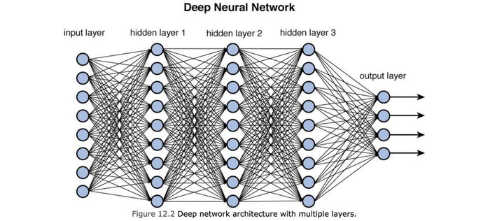
Neural Networks 101: Part 5

In this post, we are going to go into detail about Cross Entropy, Presizing and The Learning Rate Finder.

Presizing is a technique where we resize input data (mainly images) to the same size before being used as input in the Neural Network.

In previous posts, we briefly touched on why we resize images to the same size.

Cross Entropy is a loss function that is commonly used in Image Classification Models.

In previous posts, we understood loss functions in terms of a binary loss, meaning the loss is a calculation between two labels.

Cross Entropy will allow us to calculate the loss across multiple labels.

Learning Rate Finder, is a technique to find the optimum learning rate to increase the quality of adjustments when performing Back Propagation

Cross Entropy Loss

Cross Entropy Loss is a loss function that enables calculating a loss across multiple labels.

In order to understand the full picture of Cross Entropy Loss, we need to understand Softmax and the NLL (Negative Log Likelihood).

Softmax is an activation function that converts a set of values to be between 0 to 1. The whole set needs to sum to the value 1, with each value in the set representing a probability.

Negative Log Likelihood takes the outputs of the Softmax probabilities according to the targets, and applies the -log(p) to the correct probabilities.

Below we’ll go through the steps of the Cross Entropy Loss Function.

Step 1. Predictions

Predictions are calculated like in our previous blog posts. These predictions are still in its rawest form, e.g. numbers in a tensor, which we will call logits.

Step 2. Softmax Activation Function

The predictions are passed to a softmax activation function.

This activation function applies the predictions as exponents to the natural logarithm number e (2.71828).

Each exponent result is divided by the sum of all exponent results. This ensures the probabilities are distributed between 0 to 1 and all sum to 1.

We can represent each raw logit generated as a series of numbers below in a list z.

$ \mathbf{z} = [z_1, z_2, \ldots, z_n] $

We are going to take each number and apply it as an exponent to the natural logarithm e.

In order to smooth out the set of logits to predictions that must sum to 1, we will divide each exponentiated logit by the sum of all exponentiated logits.

$ p_i = \frac{e^{z_i}}{\sum_{j=1}^n e^{z_j}} $

The output will be a series of predictions that all sum to 1.

$ \mathbf{p} = [p_1, p_2, \ldots, p_n] $

Why exponentiate?

Exponentiating each prediction using a base e enures all outputs will be positive, which is required to be used as probabilities
Amplifies the differences, making bad predictions seem further apart

Step 3. Apply Negative Log Likelihood

Given a list of probabilities from the softmax function that all sum to 1, a probability is taken from the list for each specific target label. We will call this the “true” class.

This probability is then passed to a -log(p) function. Using the log function, it enhances the variance of poor probabilities e.g. a poor prediction is emphasized and aids in gradient calculation.

The negative aspect of the log function essentially inverts values to fit the format of reducing a loss function towards 0.

Below is a simple example that explains the use of negative log.

The probability p = 0.01 means the model is very unsure of a prediction, let’s assume this probability maps to the true class, it’s incorrect.

Calculating the the negative log of 0.01 gives us a loss of 4.605, since it’s very far from 0, the prediction is very imprecise.

The final output of $-log(p)$ can be seen as a high loss since its far away from 0 and gradients can be readjusted to move it closer to 0.

$ -log(0.01) = -(-4.605) = 4.605 $

If we did not apply the negative log and instead used the positive log, our output would look like below:

$ log(0.01) = -4.605 $

The negative value is difficult to use since to represent a loss, we could not subtract from it to get towards 0.

Step 4. Calculate the Mean Loss

To compute the overall loss for the batch, we take the mean of all the negative log likelihoods for the true classes.

N are the true classes
Pki is each corresponding NLL probability for the true classes
L is the calculated mean Loss

$ L = -\frac{1}{N} \sum_{i=1}^N \log(p_{k_i}) $

Learning Rate Finder

The Learning Rate Finder is a technique that was introduced by Leslie Smith.

The motivation behind the this technique is when training a model, how do we choose the optimum learning rate?

A learning rate that is too high will create large steps towards the crtiical point (the label) and will “overshoot” on each adjustment.

A learning rate that is too low will not adjust the parameters sufficiently on each step, leading to a model that is not as accurate as it could be.

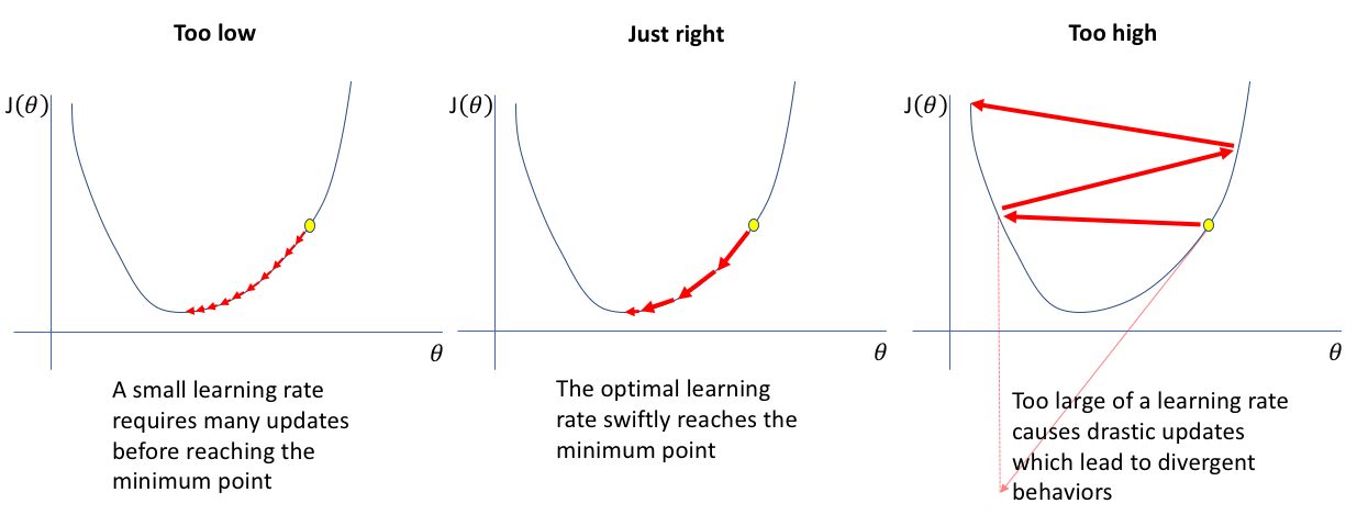
The technique involves training over a mini batch with a very small learning rate. The learning rate is gradually increased on each epoch.

The loss is recorded on each iteration. The loss should decrease on each iteration, once the loss goes up, we can determine that the learning rate will cause the steps to overshoot. Therefore, the optimum learning rate is the last value that causes the loss decrease before overshooting.

Summary

We explained and looked at the Cross Entropy Loss Function.

Cross Entropy allows the calculation of a loss across multiple labels
Cross Entropy loss uses two functions - Softmax and Negative Log Likelihood
Softmax acts as an activation function to convert logits to probabilities
Negative Log Likelihood converts the probabilities for each true class to a positive log output, the mean is calcualted and that is the loss

Below is the summary of the mathematical process

z is the generated logits

$ z = [z_1, z_2, ... z_n] $

Softmax takes the logits and converts them to probabilities. It raises each logit to the natural logirthm e
Divide each exponentiated logit by the sum of all exponentiated logits, returning a list p of probabilities
Each probability in a row must sum to 1 and represents the probability at each index mapped to the target labels