Neural Networks 101: Part 4

Understanding Layers of a Neural Network

Neural Networks are organized by “layers”. This means each layer performs a transformation on the input data using the weights and bias, applied to a function e.g. a Linear Function y = mx + b.

$ m = weights $

$ x = input data $

$ b = bias $

In between each layer, there is an Activation Function (e.g. ReLU or sigmoid) that transforms the output of the previous layer as appropriate input into the next layer.

This is important since it introduces non-linearity allowing the Neural Network to model complex patterns. Without the Activation Function, the Neural Network would become one continuous line.

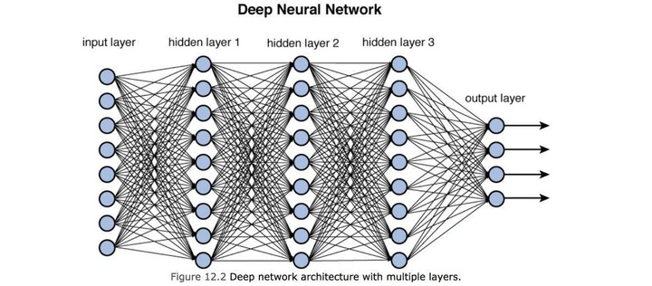
When we see visual representations of Neural Networks like in the image below, we can view each layer. Transformations on the input data are performed on the nodes and the arrows are the Activation Functions before passing the data to the next layer.

Each layer has certain terms:

• The first layer is known as the input layer, this is the layer that first handles the input data. It doesn’t perform transformations, it distributes the data into the subsequent layers
• Subsequent layers are called hidden layers, this is where the majority transformations are applied. They are called “hidden” layers since they don’t interact with the external environment (initial input or final output)
• The final layer is the output layer, this where the final prediction is delivered

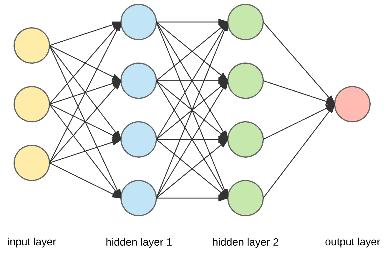
Here’s another representation of a Neural Network.

This is using Pytorch Sequential and Pytorch Linear and Pytorch ReLU.

simple_net = nn.Sequential(
    nn.Linear(PIXEL_SIZE, 30),
    nn.ReLU(),
    nn.Linear(30, 30),
    nn.ReLU(),
    nn.Linear(30, 30),
    nn.ReLU(),
    nn.Linear(30, 30),
    nn.ReLU(),
    nn.Linear(30, 30),
    nn.ReLU(),
    nn.Linear(30, 30),
    nn.ReLU(),
    nn.Linear(30, 30),
    nn.ReLU(),
    nn.Linear(30, 30),
    nn.ReLU(),
    nn.Linear(30, 30),
    nn.ReLU(),
    nn.Linear(30, 1),
)

We can see that in our simple_net there’s 9 learnable layers, represented as nn.Linear(30, x). The first layer is the input layer, so its not a learnable layer.

If we do a step through the Neural Net:

1. The Neural Network initializes the weights and bias and the input data to an output size of 30 values
2. Subsequent hidden layers will apply the weights and bias to the input data of 30 values and then output 30 values. The Activation Function will be applied to the 30 values to introduce non-linearity and the 30 values are used as input in the next layer
3. This process continuous through the layers until it reaches the final layer, the output layer. The output layer has one value, which will be our prediction

Backpropagation

If we remember in the previous blog posts, Backpropagation is the technique of calculating the gradients and then updating the weights and bias.

Using the Python code example above, Backpropagation is the movement backwards from the output to the input but using each layers output as part of the calculation of the gradient.

Different Types of Neural Networks

Feed Forward Network

The types of Neural Networks we’ve been using in these blog posts are Feed Forward Neural Networks.

Feed Forward Neural Networks are characterized as information flowing in one direction, from input to output layers. They are a straight forward type of Network since layers don’t have any loops or cycle mechanisms.

Feed Forward Neural Networks are prevelant in image recognition/classification Models.

Convolution Neural Network (CNN)

In this series of blog posts, we’ve more or less been generalizing over a Convolution Neural Network.

A CNN is a type of Feed Forward Neural Network that has been traditionally used for image classification/recognition.

Did you find this page helpful? Consider sharing it 🙌