Neural Networks 101: Part 3

This post will go through the mechanics of a Neural Network.

In Part 1 and Part 2 we went through an overview of Neural Networks and some of the maths behind the training process.

This blog post will focus specifically on understanding the mechanics of a Neural Network and is a good supporting document for the Neural Network from “scratch” notebook.

The notebook has a link to Kaggle, I recommend you follow the link and run the notebook.

I recommend using this blog post in conjuction with the Kaggle notebook to have a better understanding of the overall concepts along side the code in Kaggle.

Recap

Let’s recap our understanding of Neural Networks.

• Neural Networks are a type of computer program, capable of learning to solve complex tasks on their own

• Given some input and parameters, a Neural Network will output a prediction

• Given some prediction, a Neural Network will calculate an accuracy of the prediction, aka the loss

• A Neural Network will automtically self correct by calculating the gradient/derivatives of the loss, and updating the parameters to increase the prediction accuracy on the next iteration

Let’s recap the learning process of Neural Networks in further detail.

• Neural Networks randomly initialize the starting parameters partly due to the understanding of the Universal approximation theorem

• Predictions are calculated by the probability of a certain input matching a certain label

• The loss is calculated as metric of accuracy, basically the distance between the prediction and the correct label

• The gradient is calculated as a derivative of the prediction from the label. This gives us a variable which is the magnitude and direction towards the critical point (the correct label)

• In order to update the parameters with our gradient, we step the parameters. This means we use a learning rate as a scalar variable, and subtract the parameters according to the gradient and learning rate. This is an optimization method known as Stochastic Gradient Descent.

• We continue this process until we reach a point where the loss is at a sufficient level and we stop.

Mechanics of a Neural Network

Training, Validation and Testing sets

When it comes to training our Neural Network, we need to organize our data in to certain sets.

Training Set

This is our main dataset that will contain our input data and labels. This is the main input we are going to feed into the Neural Network. This is the dataset that will be used through the whole learning process.

Validation Set

This a dataset that is withheld from the training process. This dataset is used to gauge the accuracy and improvements of the Neural Network on each iteration.

In more detail, after creating a prediction, calculating the loss, calculating the gradients and applying the step using the training data. We use the validation set as input to the Model to measure the accuracy of predictions.

This is an important step because this acts as a good test of the current state of the Model. The Model won’t have seen these inputs before, so it’s as if the Model is making predictions on entirely new and unseen data.

Some datasets may already be split between training sets and validation sets but some may not be. In the case of a dataset not already being split, a common technique is to do a 80/20 split of the whole dataset into training/validation.

Testing Set

The testing dataset is a slightly different from the validation set.

The testing set is not used on each iteration to test the current accuracy of the Model.

The testing set is used after the training of the Model. The purpose is to test the accuracy of the Model after making big changes. For example, if we train the Model in other domain/dataset, we can use the test set to ensure the Model still performs in the original domain.

Batching

In the Kaggle book, you will notice that we batch training dataset.

This is an important method since training of Neural Networks is performed on GPUs, we need to be mindful about the the memory usage of the GPUs.

GPUs unlike CPUs, do not have its own operating system to perform memory management. It is up to the program to allocate and deallocate memory in the GPU.

Furthermore, GPUs have memory constraints, very large datasets (such as a million images) would not be able to be loaded into the GPU memory at once.

GPUs excel in parallelism, therefore, loading multiple batches of training data can speed up the training of a Model.

Activation Function

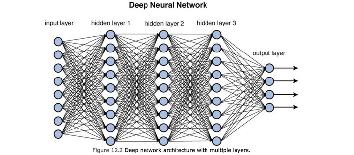
Activation Functions, are functions that connect one layer of a Neural Network to another.

Specifically, it transforms the outputs of one layer, so that it can be used as input in the next layer.

One way to think about the Activation Functions is, imagine a Neural Network as one continuous line on a graph. Many Activation Functions will act as bends, on the line, this allows the line to fit many types of models/patterns.

Activation Functions introduce “non-linearity” to the Neural Network.

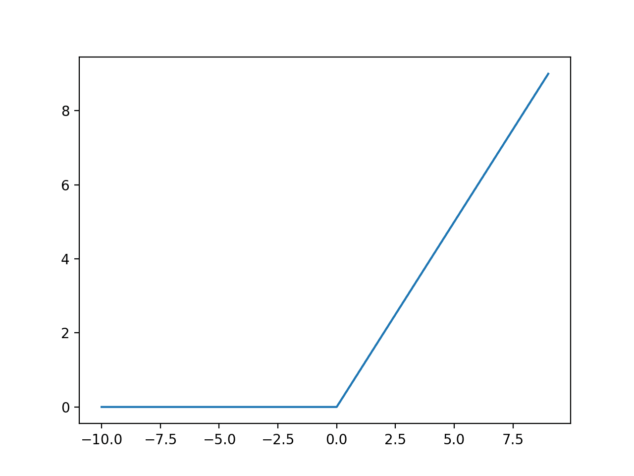
ReLU

The Rectified Linear Unit, is one type of such Activation Function.

$ f(x) = max(0, x) $

The ReLU, turns all negative input into a 0 output and allows through any positive input as output.

Sigmoid Function

The sigmoid function is another Activation Function but transforms any negative input or input over 1 into an output value between 0 and 1.

$ σ(x) = \frac{1}{1+e^-1} $

As a very inaccurate and quick example.

• If we are given a -5.00 the output of the sigmoid function might be 0.1
• If we are given a 10.00 the output of the sigmod function might be 0.9

Weights and Biases

The weights and bias are the variables in the parameters.

These variables are used to adjust the input signals across the Neural Network layers. Essentially, these variables are used to control how the Neural Network shapes the predictions.

The weights and bias are analogous to the coefficients in a linear equation y = mx + b, where the weight is m and the bias is b.

Epoch

An epoch is essentially a measure of a training cycle. For example, if we train a model for 10 epochs, this iteratively repeating or learning process 10 times.

Summary

In this blog post, we’ve identified and explained some of the mechanics of a basic Neural Network.

• The different types of datasets - training, validation and test
• Why we need to batch training data
• Why we used Activation Functions
• What are the Weights and Bias
• What Epochs are

This article should be used in conjuction with the Basic Neural Network from Scratch notebook.

Did you find this page helpful? Consider sharing it 🙌